Systema：系統的変動を超えた遺伝的摂動反応予測を評価するためのフレームワーク

ノンパラメトリックベースライン

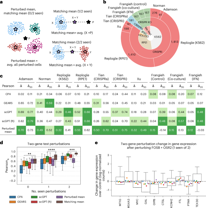
摂動平均とマッチング平均と呼ばれる2つのノンパラメトリックベースラインを設計します。

摂動平均

摂動平均は、列車セット内のすべての摂動細胞の平均遺伝子発現として、一意の摂動後のプロファイルを生成します。させて （{{ mathcal {p}}} _ {{ rm {train}}} ） 列車のセット内のすべての乱れたセルのセットになりましょう x_私 細胞の遺伝子発現になります 私。摂動平均を計算します m_パート 次のように：

このプロファイルは、すべての遺伝的摂動の予測として使用されます。

マッチング平均

一致する平均は、X+Yの組み合わせ摂動の摂動平均の拡張です。摂動後プロファイルを2つの遺伝子発現ベクターの平均として計算します （ mu（、 text {x} 、） in { mathbb {r}}}^{n} ） そして （ mu（、 text {y} 、） in { mathbb {r}}}^{n} ）、 どこ n 遺伝子の数です。させて （{{ mathcal {p}}} _ {{ rm {train}}} ） すべての列車の摂動のセットになりましょう （{ mathcal {p}}（、 text {x} 、）） 遺伝子X（または遺伝子Xの組み合わせ）が摂動された細胞のセットです。列車の時に単一遺伝子摂動xが見られた場合（x （ in {{ mathcal {p}}} _ {{ rm {train}}} ））、、 m（x）は、列車セット内のすべてのX摂動セルの平均プロファイルに対応しています。さもないと、 m（x）は、摂動平均に相当します m_パート。同様に、電車時に摂動yが見られた場合、（y （ in {{ mathcal {p}}} _ {{ rm {train}}} ））、、 m（Y）列車セット内のすべてのY摂動細胞の平均摂動に対応します。さもないと、 m（y）は、摂動平均に相当します m_パート。数学的には、マッチング平均を計算します m_{マッチング}（x、y）次のように：

単一遺伝子の摂動と組み合わせ摂動の場合、列車時に個々の遺伝子がいずれも見られなかった場合、マッチング平均と摂動平均は同等です。

摂動応答予測方法

CPAの3つの摂動応答予測方法を検討します¹⁰、ギア¹ およびscgpt² （補足情報の詳細a）。

CPAについてのメモ

CPAは、目に見えない用量と細胞型の単一細胞レベルで転写反応を予測するために設計されました。これは、この論文で検討されているシナリオとは異なります（目に見えない遺伝的摂動全体に一般化）。 CPAには、ギアとSCGPTに反して、目に見えない遺伝的摂動の転写反応を予測するメカニズムがないことを強調することが重要です。テスト時に、CPAを使用して、ランダムコントロールセルを入力としてサンプリングし、潜在空間での目的の摂動の効果を追加することにより、反事実的推論を実行しました。

評価

評価設定

単一および組み合わせの摂動を含む、目に見えない遺伝的摂動に対する一般化の評価設定を検討します。ギアのシナリオと処理ステップに従います¹、SCGPTによっても採用されました²。すべてのデータセットについて、摂動によってデータを分割し、トレーニング中に見られない遺伝的摂動の25％で構成されるテストセットを作成します。組み合わせの設定では、テスト摂動は、0/2、1/2、および2/2の目に見えない遺伝的摂動の3つのグループに分けることができます。このプロセスは、データ分割とモデルトレーニングのために異なるランダムシードを使用して3回繰り返します。したがって、我々の結果には、3つの独立した実行にわたる予測が含まれます。

微分式式プロファイルの計算

参照細胞の集団に関する平均的な発現変化を、発現プロファイルの差、または単に発現変化として参照します。数学的に、 x_私 細胞の遺伝子発現になります 私。させて （{ mathcal {p}}（、 text {x} 、）） 遺伝子X（または遺伝子Xの組み合わせ）が混乱し、許可された細胞のセットである （{ mathcal {c}} ） 参照セルのセット（たとえば、コントロールセル）になります。微分式の式プロファイルを定義します d_x 摂動xのas：

この表現は、基本的に、参照細胞の集団に関する摂動によって誘導される平均転写変化を計算します。摂動応答予測法によって推測される平均式の変化を推定するために、最初の用語は、摂動後の予測プロファイルの平均を置き換えます。

どこ （ hat {{ mathcal {p}}}（、 text {x} 、）） 特定の方法によって生成された摂動xのセルのセットと （{ hat {{ boldsymbol {x}}}} _ {i} ） 細胞の予測されるトランスクリプトームです 私。

幾何学的に、微分発現プロファイルは、参照として特定の細胞集団を使用して、同一に摂動した細胞の重心を指す高次元遺伝子発現空間のベクターに対応します（たとえば、コントロール細胞の重心）。これらのベクトルを摂動固有のシフトと呼びます。

参照ベースのメトリック

式がどれだけうまく変化するかを評価するメトリックを参照します （{ hat { delta}} _ {{ rm {x}}} ） 真の表現の変化を反映します d_x 参照ベースのメトリックとして。特に、次のギア¹ およびscgpt²、ピアソン相関係数を使用して、実際の相関関係を計算します d_x そして予測されました （{ hat { delta}} _ {{ rm {x}}} ） （1）すべての遺伝子を使用して、すべての保有摂動の発現変化（ピアソン_d）および（2）各摂動の上位20の差次的に発現した遺伝子（ピアソン_d20）。特定の摂動Xの場合、ピアソン_d20 スコアは、両方のグラウンドトゥルースからの摂動によって誘導される上位20の差次的に発現した遺伝子を選択した後に計算されます d_x と推測 （{ hat { delta}} _ {{ rm {x}}} ） 表現の変化。イチジクでの結果。 1および4は、すべての延期された摂動にわたるこれらのスコアの平均を報告します。

参照 – 感受性メトリック

参照選択の影響を受けないメトリックを参照に伴うメトリックと呼びます。たとえば、平均二乗エラー（MSE）は、数量MSE（（{ delta} _ {{ rm {x}}}、{ hat { delta}} _ {{ rm {x}}} ））参照の選択に依存しません （{ mathcal {c}} ） （参照がキャンセルアウト）。言い換えれば、微分式のプロファイルでMSEを計算する d_x そして （{ hat { delta}} _ {{ rm {x}}} ） 摂動後発現プロファイルを使用してMSEの計算に相当します。ベンチマークでは、RMSEを使用して、（1）すべての遺伝子（RMSE）と（2）各摂動の上位20の差次的に発現した遺伝子を使用して計算します（RMSE₂₀）。 RMSE₂₀ スコアは、各摂動のグラウンドトゥルースと推定された摂動後プロファイルの両方から、上位20の差次的に発現した遺伝子を選択した後に計算されます。

系統的変動に復元される参照ベースのメトリック

Systemaでは、平均oを使用して同じ評価メトリックセットを検討します_パート 参照としてのすべての摂動固有の重心O（x）のうち、摂動固有の効果を効果的に強調しています。この重心は次のように計算されます。

どこ （{{ mathcal {p}}} _ {{ rm {train}}} ） すべての列車の摂動のセット、o（x）は摂動xの重心です （{ mathcal {p}}（、 text {x} 、）） 遺伝子X（または遺伝子Xの組み合わせ）が混乱した細胞のセットです。私たちの評価フレームワークは、絶対後乱りプロファイルと摂動細胞の平均につながる原点を含むさまざまな参照選択を可能にします。

参照に敏感なメトリックの制限

摂動性重心への参照を変更すると、摂動固有の効果を強調することができますが、参照感受性メトリック（たとえば、摂動固有のシフト間のコサインの類似性またはピアソン相関）には、いくつかの制限があります。第一に、彼らのシフトの標準（参照に関して）が小さく、騒々しいターゲットにつながるため、彼らは弱い摂動を評価するのに不適切かもしれません。つまり、摂動が弱い場合、いくつかの単一の細胞の有無は、摂動固有のシフトの方向に大きな影響を与える可能性があります。参照と感受性のメトリック（たとえば、MSE）はこの制限に苦しむことはなく、最近の研究で推奨されています²⁴、しかし、解釈が比較的難しいです。第二に、参照に敏感なメトリックは、多くの場合、摂動強度に不変です。たとえば、2つのベクトル間のコサインの類似性は、その規範に依存しません。したがって、これらのメトリックは、メソッドが参照に対する摂動固有のシフトの方向を正しく予測できるかどうかを調べるために使用できますが、その大きさではありません。最後に、参照の選択は評価スコアに強く影響を与える可能性があり、特定の参照は未定義のスコアにつながる可能性があります。たとえば、摂動固有の重心が参照と重複する場合、ピアソンの相関は未定義です。要約すると、参照に敏感なメトリックは、摂動固有のシフトの相対的な方向を研究するのに役立ちます。この作業では、摂動応答の予測方法が系統的効果をキャプチャする程度を調査するためにそれらを使用しました。

重心精度

推定された摂動固有の重心が摂動の状況を正確に再構築できるかどうかを理解するために、Systemaでは、重心精度と呼ばれるメトリックを定義します。直感的には、重心精度は、摂動後の予測プロファイルが、他の摂動の重心よりも正しい地下の重心に近いかどうかを測定します。

o（x）を、根真実の式とoを使用して、摂動xの重心とします。_前に（x）予測される重心になります。させて （{ mathcal {p}} ） すべての摂動のセットになります。数学的には、重心精度は次のように定義されます。

where ({mathbb{1}}) is the indicator function and d is a predefined distance function (we used the Euclidean distance). We calculate the centroid accuracies of test perturbations. We can similarly measure the centroid accuracy with respect to a smaller set of coarse, class-specific centroids based on available perturbation annotations (for example, perturbations inducing strong vs weak chromosomal instabilities). To do so, we simply let ({mathcal{P}}) be the collection of class-specific centroids, O(X) the centroid corresponding to the class assigned to X, and O(Y) the centroid of class Y.

Gene set enrichment analysis

To identify enriched pathways (between perturbed and control cells), we performed GSEA on the processed data using GSEApy³⁰ and Biological Process 2023 gene sets from GO. We compared the populations of perturbed and control cells using signal-to-noise ratio as a ranking metric, defined as the difference of group means divided by the sum of standard deviations per group. We then ran GSEA²² with 500 random phenotype permutations (control versus perturbed) to calculate normalized enrichment scores and false discovery rates for each gene set.

AUCell

We used AUCell²³ to quantify the activity of pathways in single cells. AUCell calculates the enrichment of an input gene set as the AUC across the ranking of genes in a particular cell, leading to high scores if the gene set was enriched at the top of the ranking. This allowed us to measure whether certain gene sets were consistently enriched among perturbed or control cells.

Dataset details

Data processing

We used the codebase from GEARS¹ to process the data. We normalized each cell by total counts over all genes so that each cell has a total count equal to the median of total counts, followed by a log transformation. We discarded perturbations corresponding to genes not in the gene panel. This step is necessary for running scGPT (scGPT’s architecture was designed to handle perturbations of genes with available transcriptomic readouts). Following GEARS, we then selected the top 5,000 highly variable genes (HVGs) in each dataset¹, and included the set of perturbed non-HVGs to the gene panel. For the Replogle¹⁵ datasets, we followed the data processing strategy of scGPT²: we retained the subset of data matching the 1,973 perturbations identified in the original study¹⁵ as inducing strong transcriptional changes, and then selected 100 cells per perturbation and 2,500 control cells. In terms of Replogle¹⁵ K562, we used the genome-wide K562 perturbation screen. In terms of the Tian¹⁶ data, we discarded the perturbations PPP4R3A (SMEK1; CRISPRa dataset) and ATP5PD (ATP5H; CRISPRi dataset) that targeted only a single cell. To process the Frangieh¹⁸ data, we followed the processing steps of Lopez et al.³¹ (we first converted the data from log-normalized count per millions into raw counts and removed cells with fewer than 500 expressed genes and genes expressed in fewer than 500 cells). We then selected cells perturbed with guides that exclusively target one gene. We finally normalized the data following the standard GEARS pipeline(normalize total counts, log transformation and selection of the top 5,000 HVGs plus perturbed non-HVGs) and partitioned cells into three datasets based on their condition (control, co-culture and interferon-γ). Figure 1b reflects the number of perturbations in each dataset after processing.

Control types

All datasets used non-targeting guides as controls and the Frangieh datasets¹⁸ further incorporated intergenic guides as additional controls.

Quantification of chromosomal instabilities

We downloaded the z-scored CIN annotations from Replogle et al.¹⁵. We categorized perturbations into two groups based on the extent to which they induced chromosomal instabilities: low CIN (z-score ≤ 0) and high CIN (z-score > 2).

Annotating cell cycle

To annotate cell cycle, we utilized the Scanpy³² function scanpy.tl.score_genes_cell_cycle and the cell-cycle signatures from Tirosh et al.³³.

Reporting summary

Further information on research design is available in the Nature Portfolio Reporting Summary linked to this article.